library(tidyverse)
library(arrow) # for efficient dataframes
library(DT) # for interactive tables
library(knitr) # for tables
library(ggthemes) # for ggplot themes
library(sf) # for spatial data
library(tigris) # for US geospatial data
library(tidycensus) # for US census data
library(stargazer) # for tables
library(leaflet) # for interactive maps
options(tigris_use_cache = TRUE) # use cache for tigris
theme_set(theme_hc() + theme(axis.title.y = element_text(angle = 90))) Lab 12-1 - Next place prediction
Objectives
In this lab, we will study how simple location-based recommenders work. In particular
- We build models for the next-place prediction problem, i.e. how to make predictions of the next place a user will visit based on their previous visits.
- We will use a dataset of visits to different places in the city of Boston.
- We will use simple individual and collective models to predict the next place visited by a user.
Load some libraries and settings we will use
Load the data
We will use a dataset provided by Cuebiq that contains the visitation patterns of around 10k users in the Boston area during one month
visits <- read_csv("/data/CUS/mob10kusers.csv")
visits |> head() |> datatable()
As we can see the data contains information about the user, the CBG where the user lives (estimated), the CBG where the visit happens and the activity type of the visit. For privacy reasons, both the location and the time of the visit are up-leveled to the CBG level and the hour of the day.
Let’s change the id of the CBG to be as in the census and convert the date to R format.
visits <- visits |>
  mutate(
    HOME_CBG = ifelse(substr(HOME_CBG,1,2)=="MA",paste0("25",substr(HOME_CBG,3,12)),
                      paste0("33",substr(HOME_CBG,3,12))),
    VISIT_CBG = ifelse(substr(VISIT_CBG,1,2)=="MA",paste0("25",substr(VISIT_CBG,3,12)),
                      paste0("33",substr(VISIT_CBG,3,12))),
    TIME = ymd_hms(TIME, tz = "America/New_York"),
  )
Next place prediction
We build simple models to predict what places users will visit next. The framework will always be the same
Given a sequence of visits by users up to time \(t\) we want to build an algorithm that predicts the sequence of visits at time \(>t\).
To test the model, we will split the data into a training set and a test set. The training set will contain the first 80% of the visits and the test set the remaining 20%.
We will evaluate the model using the Accuracy@5 metric, which measures what is the fraction of the times the places in the test set are in the top 5 places predicted by our algorithm
Individual models
As we showed in the previous lectures, human mobility is very predictable and we spend most of our time in a very small number of places. Thus, just by looking at the last set of places visited by a user, we can predict the next place they will visit with high probability. This is the basic idea underneath the EPR model.
Let’s evaluate how good the model is for a particular user
user_visits <- visits %>% filter(USER == 2) |>
  arrange(TIME)
As place we use the VISIT_CBG. We will split the data into train and test and evaluate the model
set.seed(123)
train_index <- 1:(0.8*nrow(user_visits))
user_visits_train <- user_visits[train_index,]
user_visits_test <- user_visits[-train_index,]
Our predicting algorithm is very simple: for each visit, use the top-N places visited by the user in the training set to suggest new places.
topN <- function(users_visits_train, N){
  user_visits_train %>%
    count(VISIT_CBG) %>% arrange(-n) %>%
    head(N) |>
    pull(VISIT_CBG)
}
topN(users_visits_train, 5)
[1] "250173101001" "250173172033" "250173151001" "250173172031" "250092523006"And then we evaluate the model using the Accuracy@5 metric, which measures what is the fraction of the times the places in the test set are in the top-5 places predicted using the training set
mean(user_visits_test$VISIT_CBG %in% topN(user_visits_train, 5))[1] 0.6111111Let’s compute it for each user
accuracy <- visits |>
  arrange(USER, TIME) |>
  group_by(USER) |>
  filter(n() > 20) |>
  summarise(
    train_visits = list(head(VISIT_CBG, floor(0.8 * n()))),
    test_visits  = list(tail(VISIT_CBG, n() - floor(0.8 * n()))),
    top5 = list(names(sort(table(unlist(train_visits)), decreasing = TRUE)[1:5])),
    accuracy = mean(unlist(test_visits) %in% unlist(top5))
  )
ggplot(accuracy, aes(x = accuracy)) + geom_density()+
  labs(title = "Accuracy@5 for individual models", x = "Accuracy@5")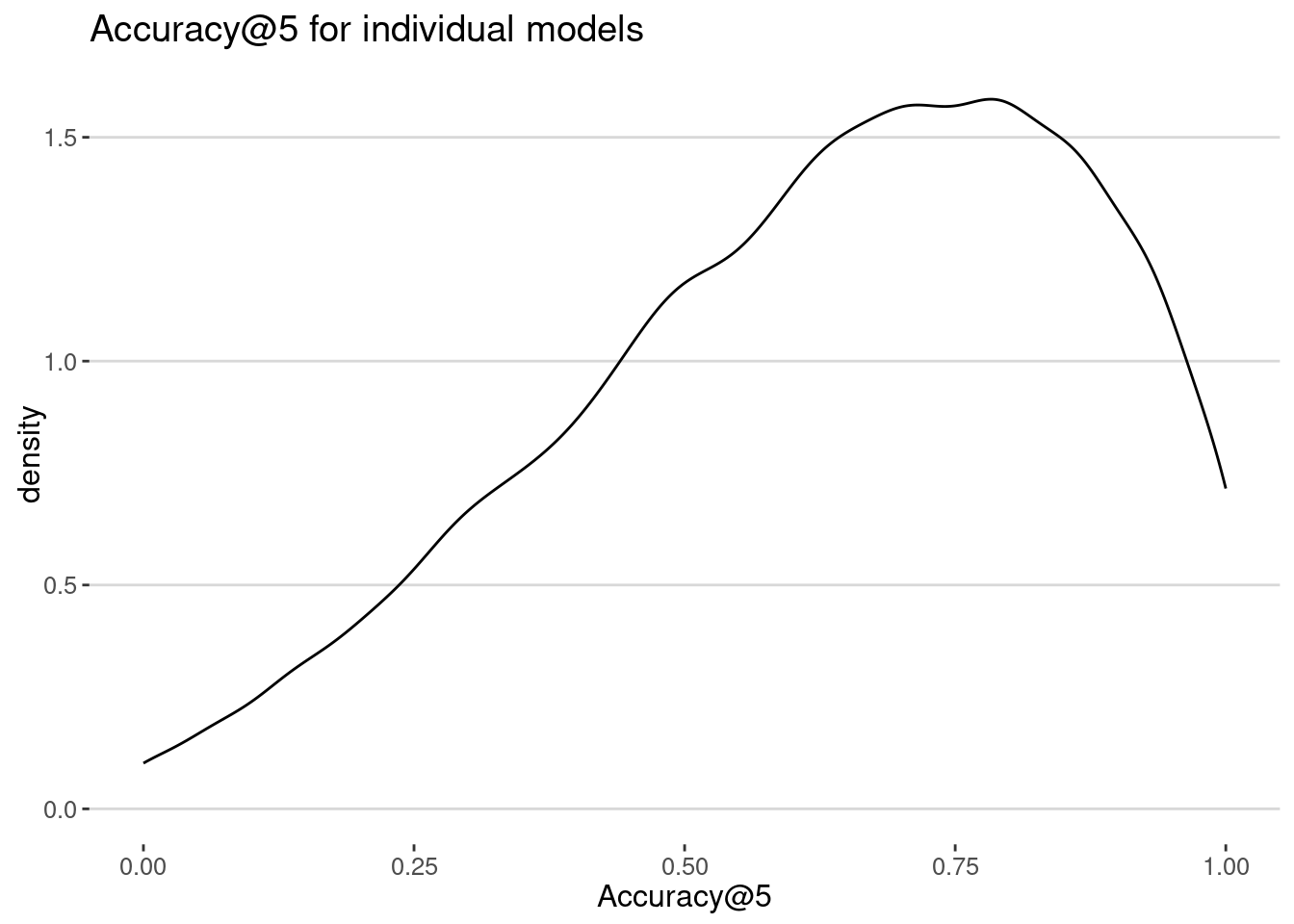
cat("Average accuracy: ", mean(accuracy$accuracy), "\n")Average accuracy: 0.6308637 As we can see the accuracy is very good, because, as we know, we tend to come back to already visited places with a high probability.
However, this model is not very useful for new places visited because it can never predict them using already visited places.
Collective models
To improve individual models, we have to start incorporating information from other users. We will start with a simple model in which we predict the next place a user visits based on the places visited by all users.
Markov model
First, we use a simple Markov model in which we assume that the next place visited depends on the last visited place, and it is given by the most likely movements of all users. In particular, let’s suppose that the user is in place \(i\) and compute the \(P_{ij}\) which is the probability that any user went from place \(i\) to place \(j\). Then, we predict that the next top-N place visited by the user is the place \(j\) that maximizes \(P_{ij}\).
We will create a matrix of transitions between places. The matrix will have a row for each place and a column for each place. The value in row i and column j will be the number of times a user visited place j after visiting place i.
transitions <- visits %>%
  arrange(USER, TIME) %>%
  group_by(USER) %>%
  mutate(is_new = if_else(!duplicated(VISIT_CBG), 1, 0)) |>
  mutate(previous_place = lag(VISIT_CBG),
         next_place = VISIT_CBG) |>
  ungroup() |>
  filter(!is.na(previous_place))
Let’s split the data into train and test. We keep the first 90% of the visits for training and the last 10% for testing
set.seed(123)
transition_train <- transitions |>
  group_by(USER) |>
  slice(1:floor(0.9*n())) |>
  ungroup()
transition_test <- transitions |>
  group_by(USER) |>
  slice((floor(0.9*n())+1):n()) |>
  ungroup()
We compute the \(P_{ij}\) matrix using the training set
transition_counts <- transition_train %>%
  count(previous_place, next_place)

transition_probs <- transition_counts %>%
  group_by(previous_place) %>%
  mutate(prob = n / sum(n)) %>%
  ungroup() |>
  arrange(previous_place, desc(prob))
Let’s check how this simple algorithm works for a particular user
transition_test_user <- transition_test |> filter(USER == 2)topN_markov <- function(current_place,transition_probs,N){
transition_probs |>
filter(previous_place == current_place) |>
arrange(previous_place, desc(prob)) |>
head(N) |>
pull(next_place)
}Let’s check it for a particular places
current_place <- c("250214563021")
topN_markov(current_place,transition_probs,5)
[1] "250214563021" "250214151024" "250214151012" "250214041002" "250235081014"We evaluate the model using the Accuracy@5 metric for just a fraction of the visits in the transition_test dataset
accuracy <- transition_test_user |>
  rowwise() |>
  mutate(next_place_pred = next_place %in% topN_markov(previous_place, transition_probs, 5))
mean(accuracy$next_place_pred)
[1] 0.8888889And now for a large fraction of the visits in the test dataset
accuracy <- transition_test |> sample_n(2000) |>
  rowwise() |>
  mutate(next_place_pred = next_place %in% topN_markov(previous_place, transition_probs, 5))
cat("Average accuracy (Total): ",mean(accuracy$next_place_pred),"+-",
    sd(accuracy$next_place_pred)/sqrt(2000),"\n")
Average accuracy (Total): 0.4735 +- 0.01116742 As we see, the accuracy is smaller than the individual model. This is because we are putting together the new places with the places visited already. Let’s see how good is the model for both
accuracy <- transition_test |>
  filter(is_new==0) |> sample_n(2000) |>
  rowwise() |>
  mutate(next_place_pred = next_place %in% topN_markov(previous_place, transition_probs, 5))
cat("Average accuracy (Returning): ",mean(accuracy$next_place_pred),"+-",
    sd(accuracy$next_place_pred)/sqrt(2000),"\n")
Average accuracy (Returning): 0.531 +- 0.01116162 and for new places:
accuracy <- transition_test |>
  filter(is_new==1) |> sample_n(2000) |>
  rowwise() |>
  mutate(next_place_pred = next_place %in% topN_markov(previous_place, transition_probs, 5))
cat("Average accuracy (Exploring): ",mean(accuracy$next_place_pred),"+-",
    sd(accuracy$next_place_pred)/sqrt(2000),"\n")
Average accuracy (Exploring): 0.095 +- 0.006558125 Remember than the accuracy of the individual model for new places is zero, so this models shows an improvement over the individual model for new places, but it is worse for returning places.
Collaborative filtering
We will use a collaborative filtering model to predict the next place visited by a user. The idea is to use the places other users visit to predict the next place a user visits.
The idea is to find a set of users that are similar to the user we want to predict the next place visited. Then, we predict the next place visited by the user as the most likely place visited by similar users.
To calculate the similarity, we construct a user \(\times\) item matrix in which items are the places visited. Since the matrix is very sparse, we use sparseMatrix in the Matrix package to store it. Since we are going to calculate the similarity between users, we select users that have some degree of activity
users_table <- transition_train |>
  group_by(USER) |>
  summarize(nvisits = n(),
            nplaces=length(unique(next_place))) |>
  filter(nvisits > 50, nplaces > 20)
Generate the sparse user-place matrix
require(Matrix)
users_table <- transition_train |>
  filter(USER %in% users_table$USER) |>
  count(USER,next_place)
users <- unique(users_table$USER)
places <- unique(users_table$next_place)
sparse_users_places <- sparseMatrix(
  i = match(users_table$USER, users),
  j = match(users_table$next_place, places),
  x = users_table$n,
  dims = c(length(users), length(places))
)
rownames(sparse_users_places) <- users
colnames(sparse_users_places) <- places
Let’s normalize each of the rows of the matrix to have a unit norm.
normalize <- function(x) {
  if(sum(x^2) > 0) {
    return(x / sqrt(sum(x^2)))
  } else {
    return(x)
  }
}
user_item_norm <- t(apply(sparse_users_places, 1, normalize))
Now we calculate the similarity between users using the cosine similarity and select for each user the 10 closest users.
\[ \text{sim}(u,v) = \frac{\sum_{i} u_i v_i}{\sqrt{\sum_{i} u_i^2} \sqrt{\sum_{i} v_i^2}} \]
To do that we use the nn2 function from the RANN package. Because we have normalized the vectors for each user, the cosine similarity is just \(sim(u,v) = 1- d_{u,v}^2/2\) where \(d_{u,v}\) is the Euclidean distance between the two vectors. Thus small distance means more cosine similarity
Let’s get the 10 users closer to each user
require(RANN)
k <- 10
neighbors <- nn2(data = user_item_norm, query = user_item_norm, k = k + 1)
# Remove the self-neighbor (first column) from the results.
neighbors$nn.idx <- neighbors$nn.idx[, -1]
neighbors$nn.dists <- neighbors$nn.dists[, -1]
Again, let’s build a function to predict the top_N new places visited by a user based on the places visited by the 10 closest users
topN_collaborative <- function(user, neighbors, N){
  #Items that the target user has visited
  user_index <- match(user, rownames(user_item_norm))
  user_items <- user_item_norm[user_index,]
  similar_users <- neighbors$nn.idx[user_index, ]
  # Get distances for these neighbors
  dists <- neighbors$nn.dists[user_index, ]

  # Compute weights using inverse distance (adding a small epsilon to avoid division by zero)
  epsilon <- 1e-8
  weights <- 1 / (dists + epsilon)

  # Weight the neighbor rows by their corresponding weights.
  # 'sweep' multiplies each row by the corresponding weight from the vector 'weights'
  weighted_matrix <- sweep(user_item_norm[similar_users, , drop = FALSE],
                           MARGIN = 1,
                           STATS = weights,
                           FUN = "*")

  # Compute recommendation scores as the column sums of the weighted neighbors
  rec_scores <- colSums(weighted_matrix)
  topN_items <- names(sort(rec_scores, decreasing = TRUE))[1:N]
  return(topN_items)
}
Let’s check how this simple algorithm works for a particular user
transition_test_user <- transition_test |>
  filter(USER == users_table$USER[200])
accuracy <- transition_test_user |>
  rowwise() |>
  mutate(next_place_pred = next_place %in% topN_collaborative(USER, neighbors, 20))
mean(accuracy$next_place_pred)
[1] 0.8888889And now for a large fraction of the visits in the test dataset
accuracy <- transition_test |>
  filter(USER %in% users_table$USER) |>
  sample_n(2000) |>
  rowwise() |>
  mutate(next_place_pred = next_place %in% topN_collaborative(USER, neighbors, 20))
cat("Average accuracy (Total): ",mean(accuracy$next_place_pred),"+-",
    sd(accuracy$next_place_pred)/sqrt(2000),"\n")
Average accuracy (Total): 0.4765 +- 0.01117078 But of course is different for returning events and exploring events
accuracy <- transition_test |>
  filter(USER %in% users_table$USER) |>
  filter(is_new==0) |> sample_n(2000) |>
  rowwise() |>
  mutate(next_place_pred = next_place %in% topN_collaborative(USER, neighbors, 20))
cat("Average accuracy (Returning): ",mean(accuracy$next_place_pred),"+-",
    sd(accuracy$next_place_pred)/sqrt(2000),"\n")
Average accuracy (Returning): 0.5895 +- 0.01100252 and for new places:
accuracy <- transition_test |>
  filter(USER %in% users_table$USER) |>
  filter(is_new==1) |> sample_n(2000) |>
  rowwise() |>
  mutate(next_place_pred = next_place %in% topN_collaborative(USER, neighbors, 50))
cat("Average accuracy (Exploring): ",mean(accuracy$next_place_pred),"+-",
    sd(accuracy$next_place_pred)/sqrt(2000),"\n")
Average accuracy (Exploring): 0.1885 +- 0.008747693 As we can see, the accuracy is higher than the Markov model.
Your turn
- Rewrite all algorithms just for visits to a category of places.
- How do the results change? Why do you think the accuracy is different?
- Which algorithm is better?
Here is the individual algorithm for Food places
visits_food <- visits |>
  filter(ACTIVITY == "Food")
Our predicting algorithm is very simple: for each visit, predict the top-N places visited by the user in the training set.
topN <- function(users_visits_train, N){
  user_visits_train %>%
    count(VISIT_CBG) %>% arrange(-n) %>%
    head(N) |>
    pull(VISIT_CBG)
}
Let’s compute the accuracy for each user
accuracy <- visits_food |>
  arrange(USER, TIME) |>
  group_by(USER) |>
  filter(n() > 20) |>
  summarise(
    train_visits = list(head(VISIT_CBG, floor(0.8 * n()))),
    test_visits  = list(tail(VISIT_CBG, n() - floor(0.8 * n()))),
    top5 = list(names(sort(table(unlist(train_visits)), decreasing = TRUE)[1:5])),
    accuracy = mean(unlist(test_visits) %in% unlist(top5))
  )
ggplot(accuracy, aes(x = accuracy)) + geom_histogram()+
  labs(title = "Accuracy@5 for individual models", x = "Accuracy@5")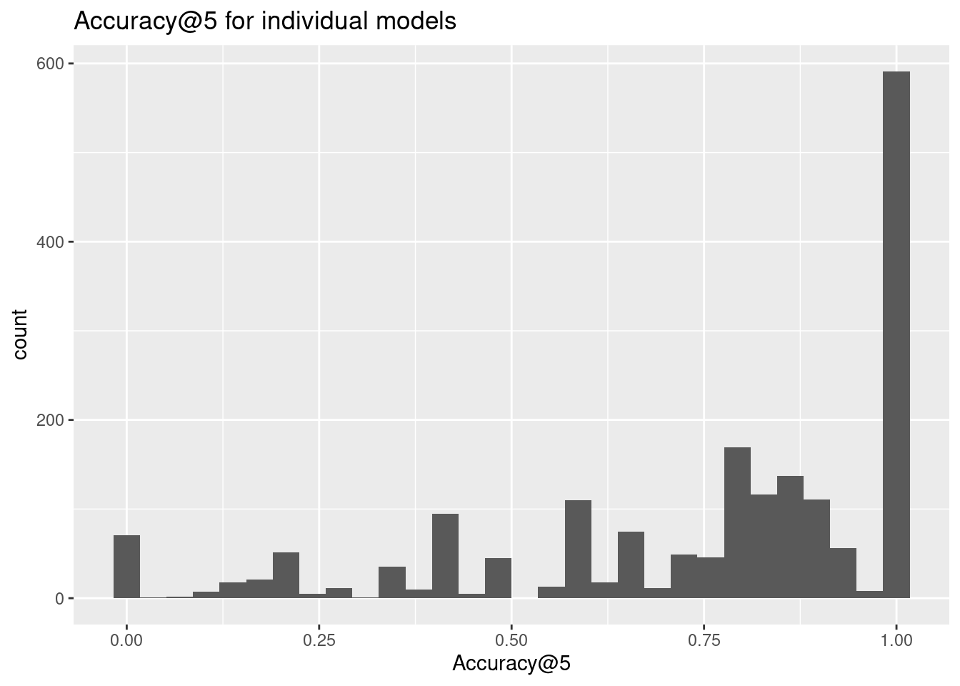
cat("Average accuracy: ", mean(accuracy$accuracy), "\n")Average accuracy: 0.7473617 Conclusions
In this lab we have seen how to build simple models to predict the next place visited by a user.
- We have seen that individual models work very well because human mobility is very predictable.
- However, these models are not very useful for new places visited by the user.
- We have seen that collective models can improve the accuracy of the predictions, specially for new places visited by the user.
- Thus, a hybrid model that combines individual and collective models could be a good approach to improve the predictions.
Further reading
Location-based recommendation Wikipedia page
Recommendations in location-based social networks: a survey by Jie Bao et al. [1]
A Random Walk around the City: New Venue Recommendation in Location-Based Social Networks by A. Noulas et al. [2]
References
[1]
J. Bao, Y. Zheng, D. Wilkie, and M. Mokbel, “Recommendations in location-based social networks: A survey,” GeoInformatica, vol. 19, no. 3, pp. 525–565, Jul. 2015, doi: 10.1007/s10707-014-0220-8.
[2]
A. Noulas, S. Scellato, N. Lathia, and C. Mascolo, “A Random Walk around the City: New Venue Recommendation in Location-Based Social Networks,” in 2012 International Conference on Privacy, Security, Risk and Trust and 2012 International Confernece on Social Computing, Sep. 2012, pp. 144–153. doi: 10.1109/SocialCom-PASSAT.2012.70.