Lecture 5-1
Statistical Analysis
of Urban Data
2026-02-09
Welcome!
This week:
Statistical Analysis of Urban Data
Key takeaway: proximity and adjacency

A tale of two cities: London’s rich and poor in Tower Hamlets
Key takeaway: proximity and adjacency
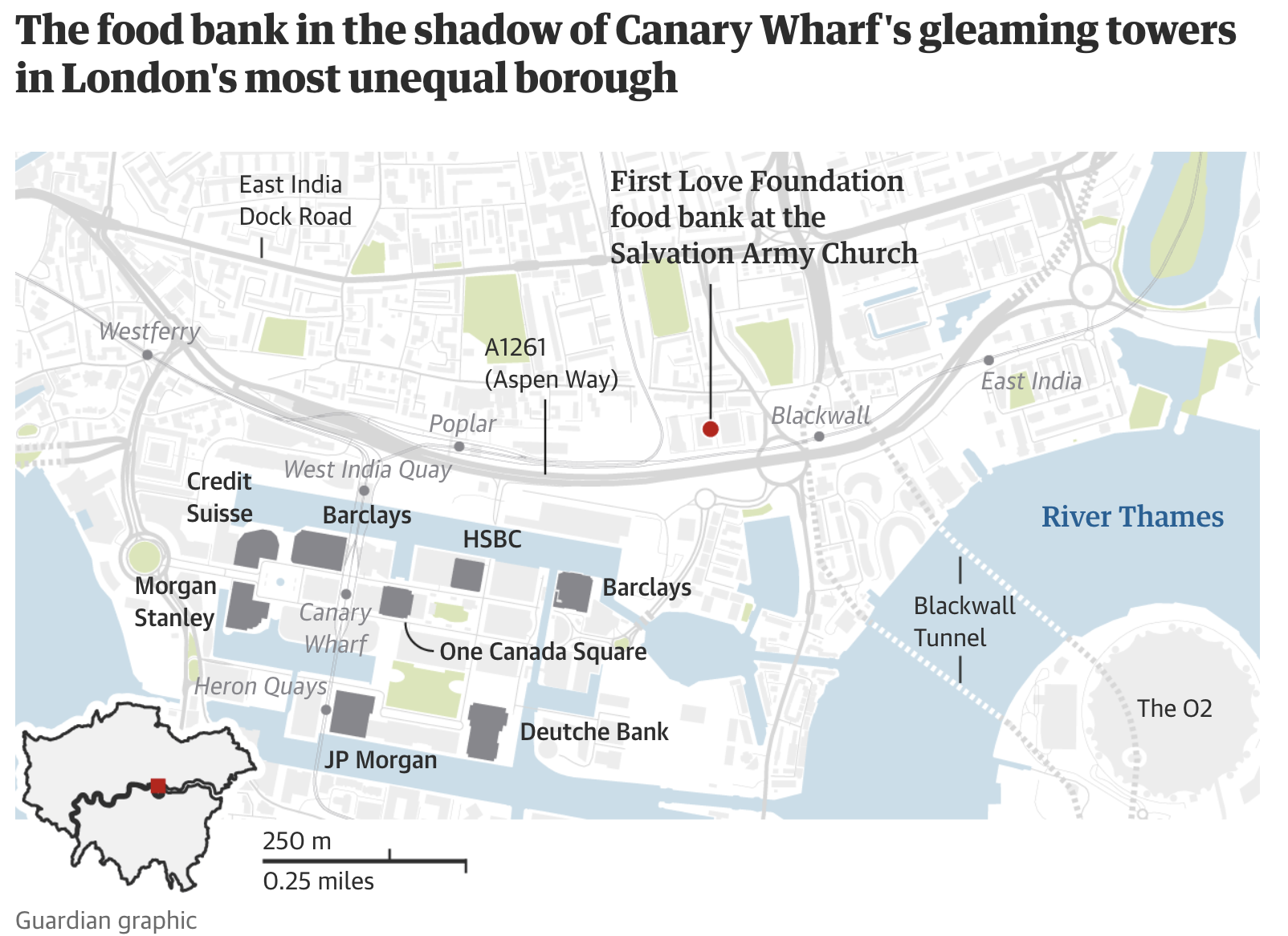
A tale of two cities: London’s rich and poor in Tower Hamlets
Spatial autocorrelation
Tobler’s first law revisited: “…near things are more related than distant.”
This is an empirical observation which holds true for a wide range of spatial phenomena.
Spatial autocorrelation permits:
- Prediction / interpolation based on physical proximity.
Spatial autocorrelation hinders:
- Statistical inference (independence assumptions are violated for most spatial data)

Spatial autocorrelation
A funny example: Inverse-distance Weighting (IDW) (1965) beats Google Research’s [1] elevation predictions:
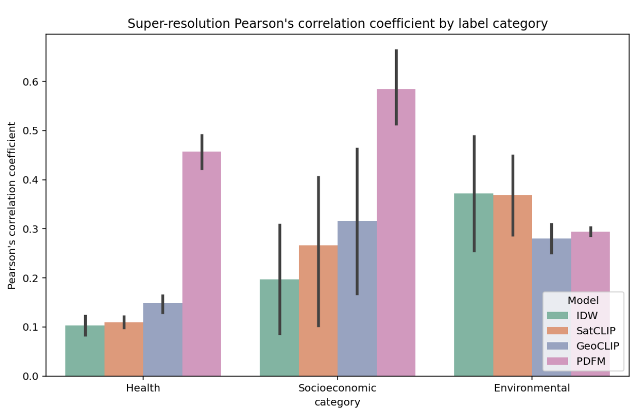
General Geospatial Inference with a Population Dynamics Foundation Model [1]
Measuring spatial autocorrelation
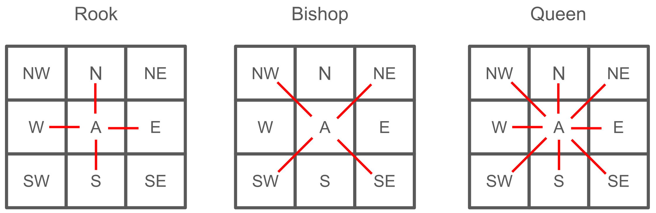
Most spatial statistics depend on a spatial weights matrix \(W\). It encodes which spatial units are considered neighbors.
Formally
- \(w_{ij}\) measures the influence of location \(j\) on location \(i\)
- Usually \(w_{ij} > 0\) if locations \(i\) and \(j\) are neighbors, else \(w_{ij} = 0\)
- Often \(w_{ii} = 0\) (a location does not influence itself)
- Often row-standardized: \(\sum_j w_{ij} = 1\) for all \(i\)
There are many ways to define neighbors. For example these are the “contiguity-based” ones
Measuring spatial autocorrelation
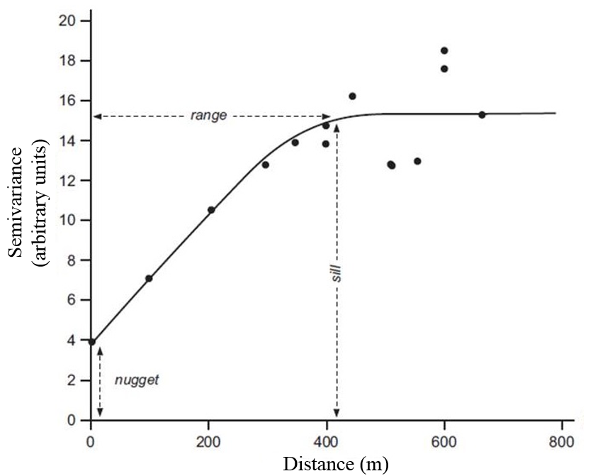
Spatial variogram: how much do two observations vary by distance?
Useful for assessing degree of spatial autocorrelation of continuous spatial variables.
\[\gamma(h) = \frac{1}{2N(h)} \sum_{i=1}^{N(h)} (z(x_i) - z(x_i + h))^2\]
Measuring spatial autocorrelation
Moran’s I
- Measures how much a value at one location is correlated with values at nearby locations.

Measuring spatial autocorrelation
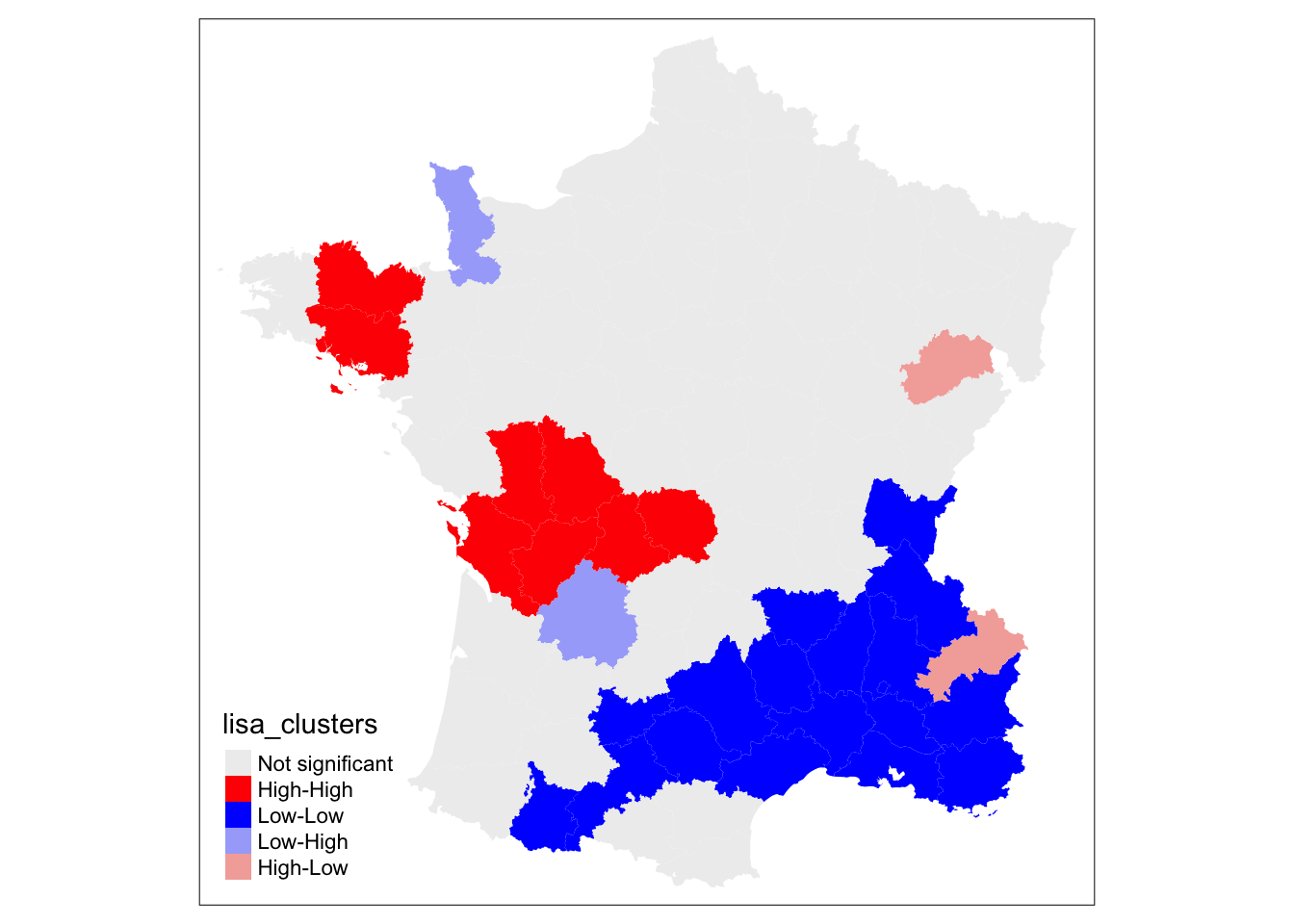
Local Indicators of Spatial Association (LISA)
- Local version of Moran’s I, assigned to each area and compared to an area’s neighbors [2].
- LISA results are expressed as the the value of a spatial variable relative to neighbors and the global mean:
- “High-High” or “Low-Low” (High / Low local value with High / Low values of neighbors - i.e. spatial clusters)
- “Low-High”, “High-Low” (High / Low local value with Low / High values of neighbors - i.e. spatial outliers)
Warning: Edge / Boundary Effects
Most geostatistical analysis happens within a constrained spatial boundary
For proximity- or adjacency-based statistical methods (like GWR):
- Boundary locations can show spurious statistical relationships because of a lack of neighbors in the adjacency matrices used to parameterize models
Spatial clustering
Spatial clustering techniques account for spatial proximity when defining clusters.
Supports varying cluster density (producing varying size clusters).
Spatial clustering is useful for: dimensionality reduction of spatial features and for detecting spatial outliers.
In practical 5-1: note the difference between K-means clusters and geographically contiguous SKATER clusters (SKATER accounts for spatial proximity).

DBSCAN - Density Based Spatial Clustering of Applications with Noise
Spatial clustering algoritms
Most common spatial clustering algorithms:
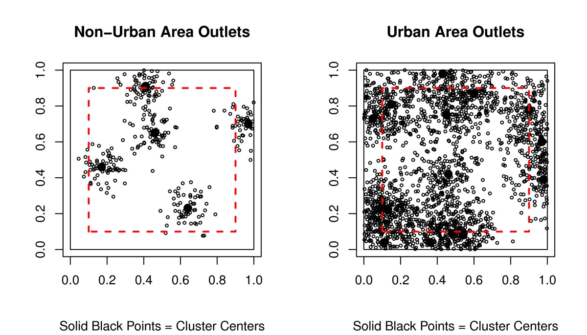
- DBSCAN [3] [4]
- Defined by two variables:
- \(minPts\): Minimum density of points defining core points (cluster centers).
- \(\varepsilon\) Maximum distance required to define border points connected to core points with neighbors \(< minPts\).
- Outliers are \(> \varepsilon\) distance from core points.

For \(minPts = 4\), \(\varepsilon\) indicated by circle radius. Red: core points, Yellow: border points, Blue: outlier.
Spatial clustering algoritms
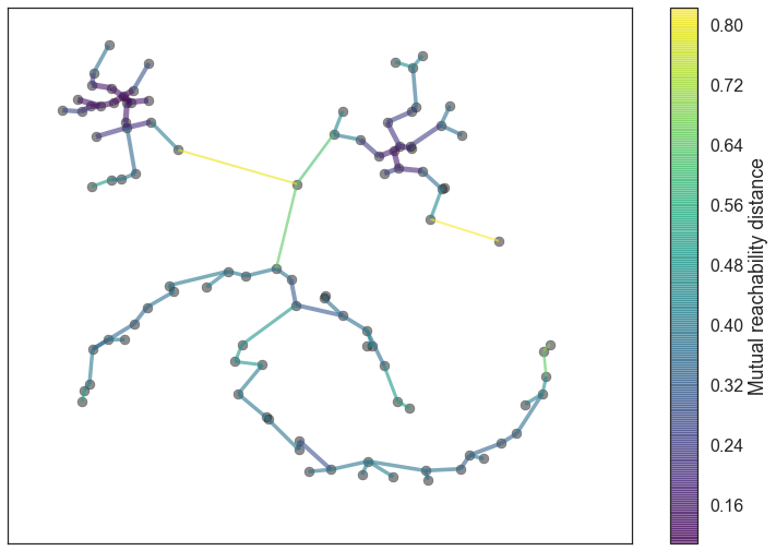
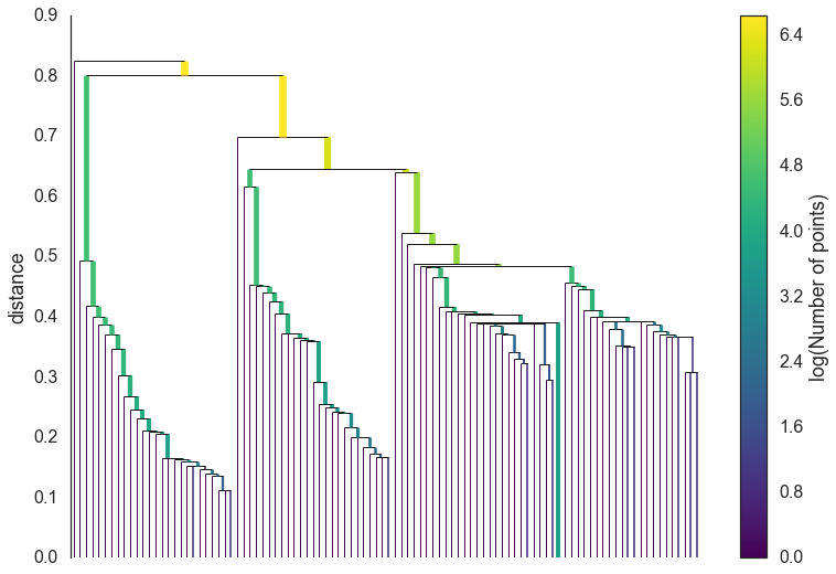
- HDBSCAN
- Replaces a single \(\varepsilon\) for a range of distance values defined by a minimum spanning tree of mutual reachability between each data point and its \(minPts\) nearest neighbors.
Geodemographic analysis
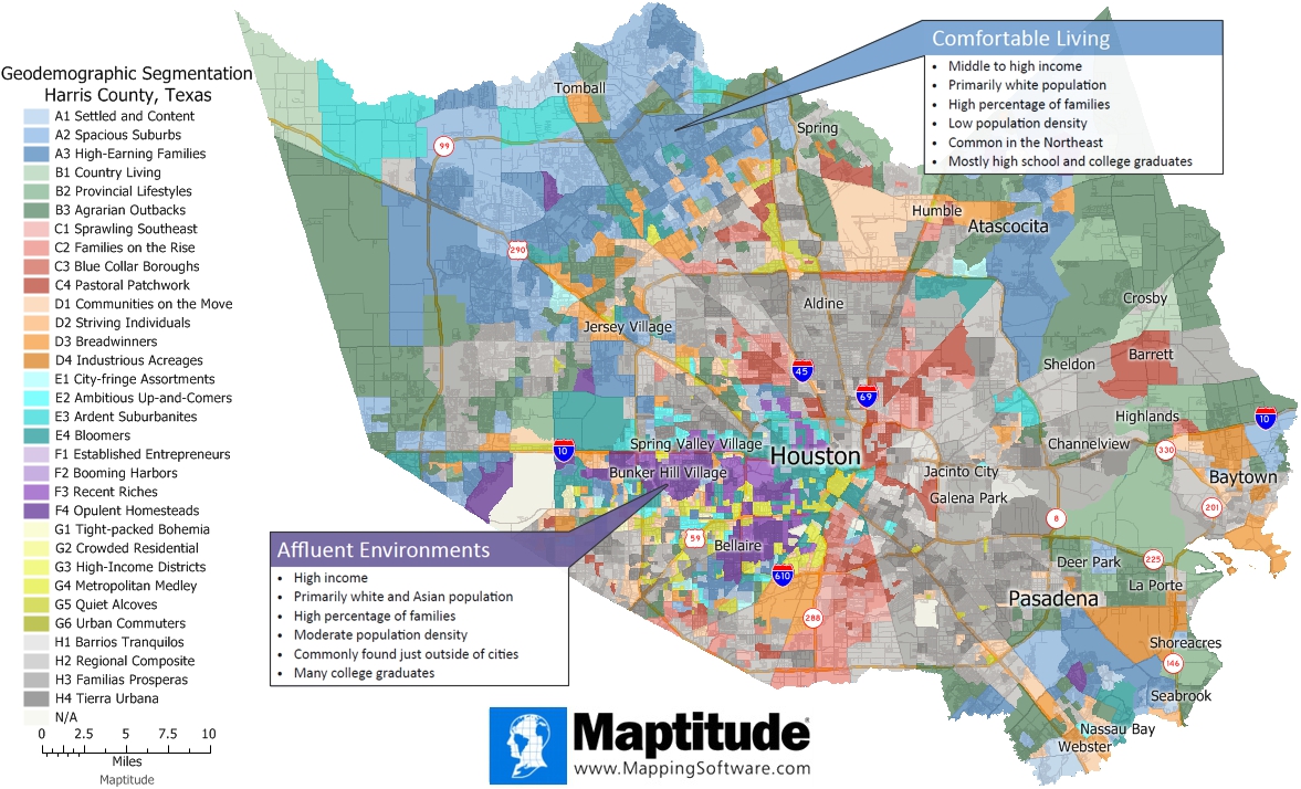
From Maptitude
Geodemographic analysis
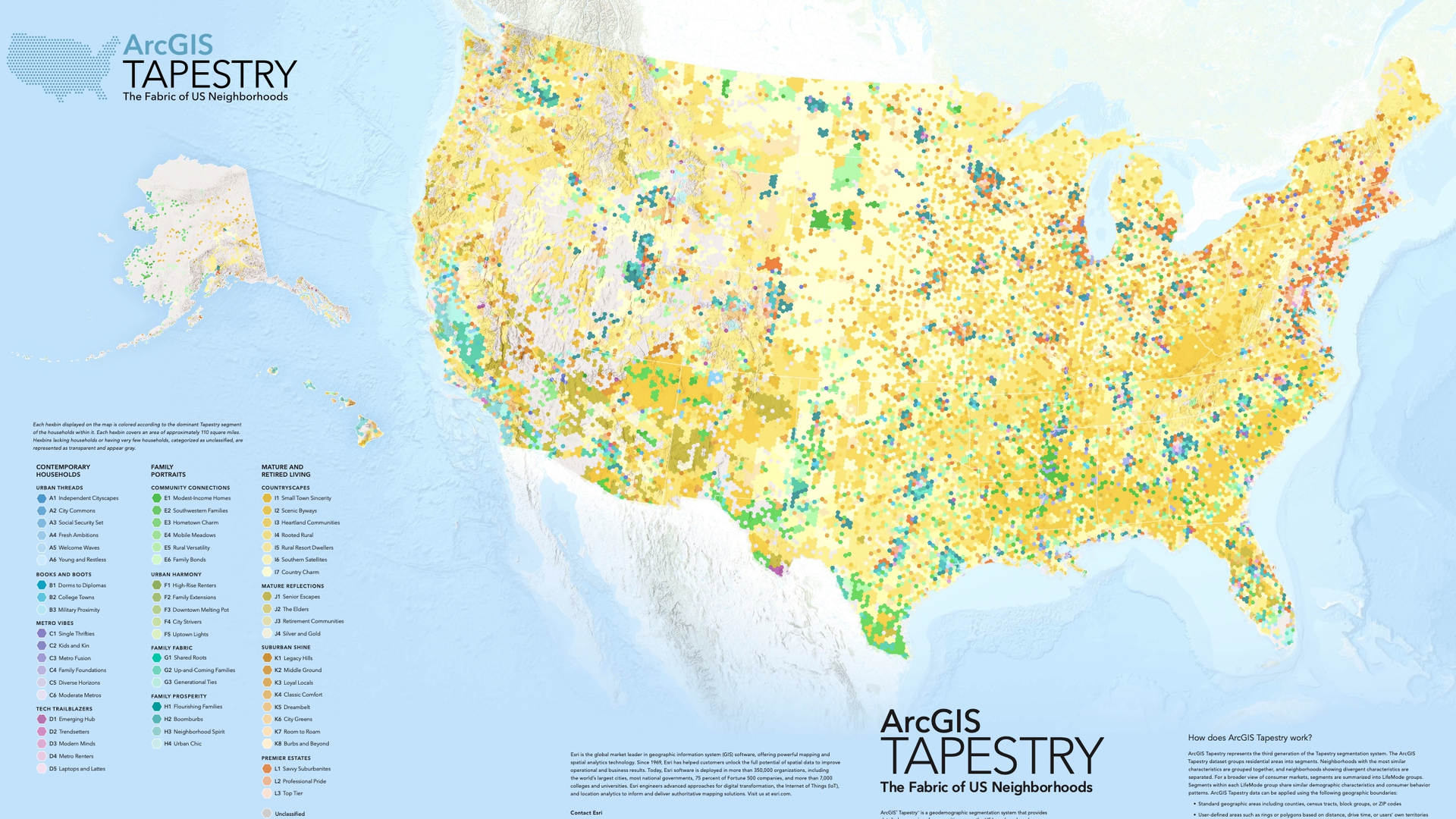
From ESRI Tapestry
Geodemographic analysis

From ESRI Tapestry
References
![]()