library(tidyverse)
library(arrow)
options(arrow.unsafe_metadata = TRUE)
library(sf) # for spatial data
library(tigris) # for US geospatial data
library(leaflet) # for interactive maps
library(ggthemes)
theme_set(theme_hc() + theme(axis.title.y = element_text(angle = 90))) Lab 5-2 - Detecting Hotspots in Urban Areas
Objective
In this practical, we will use spatial clustering techniques (dbscan) to identify “hotspots” in urban areas. IN particular, we will:
- Use the Foursquare POIs dataset in a city
- Run DBSCAN and HDBSCAN to find hotspots.
- Choose parameters and evaluate the results.
- Map clusters and interpret them
Load some libraries and settings we will use
Load the FSQ POIs daset
files_path <- Sys.glob("/data/CUS/FSQ_OS_Places/places/*.parquet")
pois_FSQ <- open_dataset(files_path,format="parquet")
pois_FSQ |> head() |> collect()# A tibble: 6 × 23
fsq_place_id name latitude longitude address locality region postcode
<chr> <chr> <dbl> <dbl> <chr> <chr> <chr> <chr>
1 4aee4d4688a04abe82d… Cana… 41.8 3.03 Anselm… Sant Fe… Gerona 17220
2 cb57d89eed29405b908… Foto… 52.2 18.6 Mickie… Koło Wielk… 62-600
3 59a4553d112c6c2b6c3… CoHo 40.8 -73.9 <NA> New York NY 11371
4 4bea3677415e20a110d… Bism… -6.13 107. Bisma75 Sunter … Jakar… <NA>
5 dca3aeba404e4b60066… Grac… 34.2 -119. 18545 … Tarzana CA 91335
6 505a6a8be4b066ff885… 沖縄海邦… 26.7 128. 辺土名130… 国頭郡国頭村…… 沖縄県 <NA>
# ℹ 15 more variables: admin_region <chr>, post_town <chr>, po_box <chr>,
# country <chr>, date_created <chr>, date_refreshed <chr>, date_closed <chr>,
# tel <chr>, website <chr>, email <chr>, facebook_id <int>, instagram <chr>,
# twitter <chr>, fsq_category_ids <list<character>>,
# fsq_category_labels <list<character>>Choose a city
city_location <- "Boston"
pois_city <- pois_FSQ |> filter(locality == city_location & region == "MA") |> collect()
pois_city <- pois_city |> filter(!is.na(longitude) & !is.na(latitude))
nrow(pois_city)
[1] 56747Convert to sf and project to meters (UTM).
pois_city_sf <- st_as_sf(pois_city, coords = c("longitude", "latitude"), crs = 4326) Visual sanity check
pois_city_sf |> sample_n(5000) |>
  leaflet() |>
  addProviderTiles("CartoDB.Positron") |> addCircles()
As we can see from the map, there are many POIS outside of the city limits. Let’s get the city limits from the Census and filter to only those POIs inside the city.
city_limits <- places(state = "MA", cb = TRUE, progress=F) |>
  filter(NAME == city_location) |>
  st_transform(crs = st_crs(pois_city_sf))
pois_city_sf <- pois_city_sf |> st_join(city_limits, join = st_within) |> filter(!is.na(NAME))
Sanity check, plot the pois and the limits of the city
pois_city_sf |> sample_n(5000) |>
  leaflet() |>
  addProviderTiles("CartoDB.Positron") |>
  addCircles() |>
  addPolygons(data = city_limits, color = "red", weight = 2, fill = FALSE)
Run DBSCAN
DBSCAN / HDBSCAN are density-based clustering algorithms that can be used to identify clusters of points in space. They are particularly useful for spatial data because they can find clusters of arbitrary shape and do not require the number of clusters to be specified in advance.
They need distances in meters, so we will project our data to UTM.
pois_city_sf_utm <- st_transform(pois_city_sf, crs = 32619) # UTM zone 19NNow we can run DBSCAN. We need to choose two parameters:
eps(the maximum distance between two points to be considered neighbors) andminPts(the minimum number of points required to form a cluster).
library(dbscan)
set.seed(123)
minPts <- 20
dbscan_result <- dbscan(st_coordinates(pois_city_sf_utm), eps = 100, minPts = minPts)
pois_city_sf_utm$dbscan_cluster <- dbscan_result$cluster
Now we can visualize the clusters.
pois_city_sf_utm |>
  filter(dbscan_cluster != 0) |>
  ggplot() +
  geom_sf(aes(col=factor(dbscan_cluster))) +
  theme_void() +
  labs(color = "DBSCAN Cluster") +
  ggtitle("DBSCAN Clusters of POIs in Boston")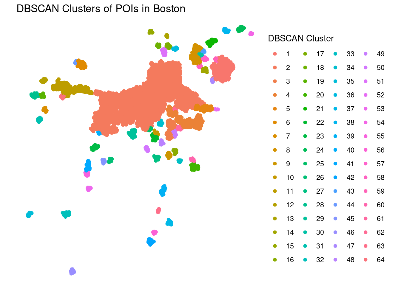
As we can see, DBSCAN has identified several clusters of POIs in the city, but most of the points belong to the first cluster (cluster 1). This is a common issue with DBSCAN, as it tends to create one large cluster and several small ones.
One possibility is to work with the eps parameter. To do that we can check how far are minPts nearest neighbors for each point using different radiuos eps
kdist <- dbscan::kNNdist(st_coordinates(pois_city_sf_utm), k = 20)
plot(
  sort(kdist[kdist>0]),
  log = "xy",
  xlab = "Points (rank, log scale)",
  ylab = "20-NN distance (meters, log scale)",
  main = "k-distance plot (log–log)"
)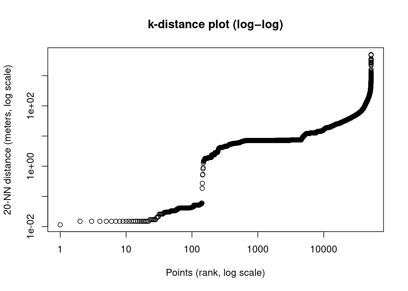
Each point shows the distance to its 20th nearest neigbhor, sorted from smallest to largest. We can see different structures of the data:
- A dense region with small distances (centimiters to meters), probably POIs packed into the same buildings/blocks
- Urban fabric, middle distances (100-300 meters), probably POIs in the same street or block
- Sparse region with large distances (> 300-500 meters), Suburban, industrial, isolated POIs. These points becomes noise under DBSCA
Exercise
- Which
epsvalue would you choose? Try different values and see how the clusters change.
HDBSCAN
As we have seen, DBSCAN requires one eps, but cities have multiple densities. Downtown is dense, but suburban areas are sparse.
HDBSCAN is a hierarchical version of DBSCAN that can find clusters of varying densities. The idea is to build a hierarchy of clusters based on the density of points, and then extract the most stable clusters from this hierarchy. We select only 20k points for speed
set.seed(123)
pois_city_sf_utm_sample <- pois_city_sf_utm |> sample_n(20000)
hdbscan_result <- hdbscan(st_coordinates(pois_city_sf_utm_sample), minPts = 20)
Let’s see the results
table(hdbscan_result$cluster)
   0    1    2    3    4    5    6    7    8    9   10   11   12   13   14   15
9098   20   95   42   59   45   44 1091   39  175   39   66   23   21   46   37
  16   17   18   19   20   21   22   23   24   25   26   27   28   29   30   31
  39   20   46   50   27   91   61   26   33   66   74   26   38   41   81   31
  32   33   34   35   36   37   38   39   40   41   42   43   44   45   46   47
  25   24   60   76   91   46   25   24   80   55  124   28   93   28   28   24
  48   49   50   51   52   53   54   55   56   57   58   59   60   61   62   63
  47  219   28  103   37   27   33  196   54  318   68   22   64   37   68   33
  64   65   66   67   68   69   70   71   72   73   74   75   76   77   78   79
  26   32   64   47   53   32   40   34   23   35   43   27   61   40   89  230
  80   81   82   83   84   85   86   87   88   89   90   91   92   93   94   95
  31   32   97  120   39   20   54   42   71   25   29  191  183  137   35   58
  96   97   98   99  100  101  102  103  104  105  106  107  108  109  110  111
  29  261   58  223  113   49   27   28   20   33   49   20   83   20   25   39
 112  113  114  115  116  117  118  119  120  121  122  123  124  125  126  127
  24   54   30   53   83   33   84   25   30   79   46  138   29   34   54   29
 128  129  130  131  132  133  134  135  136  137  138  139  140  141  142  143
  26   35   22   56   51   63   52   31   24  100   31   38   36   54   63   45
 144  145  146  147  148  149  150  151  152  153  154  155  156  157  158  159
  40   25   50   50   28   50   21   29   46   20   78   54   21   44   23   25
 160  161  162  163  164  165  166  167  168  169  170  171  172  173  174
  34  202   68   22   27   81   84   34   34   27   35   45   45   75   39
As we can see HDBSCAN has identified several clusters of varying sizes, and it has also labeled 9098` points as noise (cluster 0).
HDBSCAN also assings each pont and outlier score that indicates how much of an outlier is a point: low score (0) means that it is a core point, deeply embedded in a cluster, while high-score (1) is a borderline or isolated point. We can use this score to filter out points that are not part of any cluster.
Let’s map the cluster
pois_city_sf_utm_sample <- pois_city_sf_utm_sample  |>
  mutate(hdbscan_cluster = hdbscan_result$cluster,
         hdbscan_outlier_score = hdbscan_result$outlier_scores)
Plot the data (without legend for better visualization):
library(colorspace)
pois_plot <- pois_city_sf_utm_sample |>
  filter(hdbscan_cluster != 0 & hdbscan_outlier_score < 0.8) |>
  mutate(hdbscan_cluster = factor(hdbscan_cluster)) |>
  st_transform(4326)

n_clusters <- nlevels(pois_plot$hdbscan_cluster)

pal <- colorFactor(
  palette = qualitative_hcl(n_clusters, palette = "Dark 3") |> sample(),
  domain  = pois_plot$hdbscan_cluster
)

leaflet(pois_plot) |>
  addProviderTiles("CartoDB.Positron") |>
  addCircleMarkers(
    radius = 5,
    stroke = FALSE,
    fillOpacity = 0.7,
    color = ~pal(hdbscan_cluster)
  )
As we can see, HDBSCAN has identified several clusters of varying sizes. The clusters are more balanced than DBSCAN, and they capture different densities in the city.
Exercise.
- Try different values of
minPtsand see how the clusters change. - Try filtering points with different
hdbscan_outlier_scorethresholds and see how the clusters change. - Identify the most important clusters in the city and try to interpret them. What kind of places do they represent? Are they downtown areas, commercial zones, residential neighborhoods, etc.?